Session 2
Implementing a 2D simulation of Active Brownian Particles (ABP) in C++
In the second session of this tutorial we port the Python code developed in Session 1 to C++ and build a binding of the C++ to Python. We keep the structure and naming the same as in the Python version and only make changes where necessary to set the stage for the GPU implementation in Session 3.
Brief overview of the design layout
The image below shows key components of a particle based simulation code and how they interact with each other:
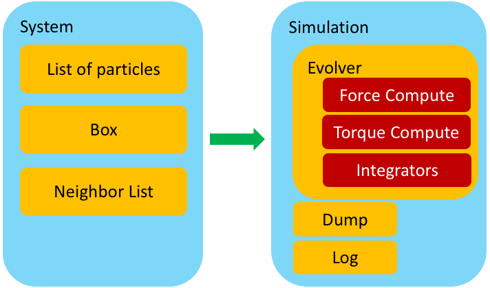
Let us briefly focus on the Evolver class. Its task is to evolve the system by a single time step, i.e., to propagate the system in time for $\delta t$. In particular, its task is to:
- Ensure that the neighbor list is up to date;
- Perform the integration pre-step;
- Compute all forces and torques on each particle;
- Perform the integration post-step;
- Apply periodic boundary conditions.
In our design, one can have multiple force and torque laws present in the system. In addition, multiple integrators can act in the same system.
Here we focus on the item 3, and, in particular, the fact that in a given system one could have multiple types of interactions.
For example, in the case we studied in Session 1, we apply the self-propulsion force, $\mathbf{F}^\text{sp}_i = \alpha \mathbf{n}_i$ on each particle. In addition, each particle experiences soft-core repulsion due to overlaps with its neighbors, i.e., $\mathbf{F}_{i}^{\text{elastic}} = \sum_j k\left(2a - r_{ij}\right)\hat{\mathbf{r}}_{ij}$ for $r_{ij} \le 2a$, with the same meaning of parameters as used in Session 1. In our implementation, each term in the total force is implemented as a separate class. The self-propulsion term is handled by the SelfPropulsion class, while the soft-core repulsion is implemented in the HarmonicForce class.
The Evolver class has a member variable called force_computes, a Python list that stores all different types of interactions used in a given simulation. To be a bit more technical, if we want to add self-propulsion and soft-core repulsion to our system, we simply create two objects (instances), one for each of the two "force type" classes and append them to the force_computes list of the Evolver class.
The evolve function of the Evolver class then simply iterates over all elements of the force_computes list and calls the appropriate compute function for each element.
It is not a coincidence that we put the word simply in bold. Due to Python's expressive and powerful data structure this was all we needed to do. However, a lot of things are happening under the hood here, which we need to understand if we are to switch to C++. Code written in C++ is in general much faster than the same code written in Python. This, however, comes at the expense that a lot of things that "just work" in Python, need to be explicitly implemented in C++.
In order to understand how to port to C++ the same functionality that allows us to split different types of forces into separate classes, we need to introduce the concepts of class inheritance and smart pointers.
Classes
Class is the central language feature of C++. It is a user-defined type that represents a concept in the code. An instance of a class is called an object. A typical class is, therefore, a piece of C++ code that contains some data (called member data) and some operations that are performed on that data (called member functions). It also specifies how instances of the class are created (i.e., constructed) and how object intact with the environment. In other words, a class is an abstraction of a set of properties and operations that can be performed on those properties. Note that a class can contain members only (i.e., no member functions) but it also can contain no member data and only member functions. At first, the later example sounds paradoxical but it is of central importance for this discussion.
Concrete classes
Let us give several concrete examples of classes.
One of the central entities in our simulation is a particle. It is, therefore, natural to represent it as a class. This is a very simple class that holds basic information such as position, velocity, type, etc. of a particle.
struct Particle
{
    int id;           // particle id
    int type;         // particle type
    real radius;      // particle radius
    real2 r;          // particle position
    real2 v;          // particle velocity
    real2 f;          // particle force
    real2 n;          // particle director
};
Arguably, Particle is not an overly exciting class as it does not do much. A more interesting example is the System class. This class hold the list of all particles and basic operations on them, such as adding a new particle. In a reduced form, this class could look something like this:
class System
{
public:

    System(Box& box) : _box{box}, _numparticles{0} { _particles.clear(); }
    ~System() { }
    std::vector<Particle>& get(void) { return _particles; }
    void add_particle(const Particle& _particle)
    {
        _particles.push_back(_particle);
        _particles[_numparticles].id = _numparticles;
        _numparticles = _particles.size();
    }
    int size() const { return _numparticles; }

private:

    Box& _box;                           // Simulation box
    std::vector<Particle> _particles;    // Standard library vector containing all particles
    int _numparticles;                   // Total number of particles in the system


};
Our System class is an example of a concrete class. It essentially behaves as any built-in type since it contains the data (e.g., a Standard Template Library vector of all particles) and some operations on that data (e.g., adding a new particle).
Abstract classes
What about forces though? We gave several examples of forces (e.g., self-propulsion and soft-core repulsion). These are all, however, specific examples of a force. The question is if there is a way to abstract the notion of a force and instead define an interface to all possible (within reason!) forces, some of which we may want to implement in the future?
The answer to that is provided by the concept of an abstract class. An abstract class is an interface, i.e., it is impossible to create an object that is an instance of an abstract class. However, it is possible to inherit from it and create a class hierarchy with children classes (ofter referred to as derived classes) that share the same interface as the parent class (often referred to as the base class) and provide a specific implementation. This allows us to create a robust system that can handle the entire class hierarchy and to add new functionality without having to make changes to the code that uses this class hierarchy.
At this point, this all sounds rather convoluted. So, the best is to proceed with an example.
Let us create an abstract class called Force that will serve as the interface to all forces types (for simplicity, let us restrict to single-particle and pair-wise interactions).
class Force
{
public:

    Force(System& sys) : _sys{sys} { }
    virtual ~Force() { }
    std::string get_name() const { return _name; }
    virtual void compute() = 0;

protected:

    System& _sys;       // System object
    std::string _name;  // Name of the interaction type (e.g., harmonic)
};
The Force class looks like any other class, with the exception of several important differences. The first one is that two of its member functions have a prefix virtual. This means that these functions will be overwritten by children classes and the precise version of the member function which is executed will be determined at the runtime. We will get back to this point shortly.
In addition, we have this somewhat strange line
virtual void compute() = 0;
the "=0" notation means that the compute function is a pure virtual function, i.e., just a name holder. Any attempts to call Force::compute() will result in a compilation error. This just reflects the fact that one cannot simply compute a force without knowing what that force is.
Finally, we note that the keyword protected means that those data members will be accessible by the children classes.
Class inheritance
Let us now implement a specific type of interaction, say, self-propulsion. We will do this by defining a class SelfPropulsionForce that is a child of the abstract class Force, i.e., class SelfPropulsionForce inherits the interface from the base class Force.
class SelfPropulsionForce : public Force
{
public:

    SelfPropulsionForce(System& sys, double alpha = 1.0) : Force{sys}, _alpha{alpha} { }
    ~SelfPropulsionForce() override { }
    void compute() override
    {
        for(auto& p : _sys.get())
        {
           p.f += _alpha*p.n;
        }
    }

private:

    double _alpha;   // strength of the self propulsion force
};
In the last example, line
class SelfPropulsionForce : public Force
means that the class SelfPropulsionForce is a child of the abstract class Force, i.e., it inherits its interface and some of its properties. The keyword override tells to C++ that this class "overrides", i.e., implements the actual computation of, in this case, self-propulsion force.
The power of building class hierarchies lies in how we can use the interface defined in the base class to access the children.
Let us look into the relevant part of the Evolver class, i.e., the part that stores and computes all forces.
class Evolver
{
public:

    //..
    void add_force(const std::string name, std::unique_ptr<Force> f)
    {
        // ...
        _force_list[name] = std::move(f);   // Move is used here to transfer ownership of the unique_ptr f
        // ...
    }
    //...
    void compute_forces()
    {
        for (const auto& force : _force_list)
            force.second->compute();
    }
    // ...

private:

    std::map<std::string, std::unique_ptr<Force>> _force_list;    // list of all the pointer to the forces

};
Let us analyze this example. First we note the line
std::map<std::string, std::unique_ptr<Force>> _force_list;
which tells the Evolver class to store all force types into a map (i.e., loosely speaking, a C++ version of Python's dictionary) where keys are strings (i.e., the name of the force, such as 'self-propulsion') and the value is a unique pointer to the Force object.
There are two important points in here. A unique pointer is a version of a smart pointer. A smart pointer is a close cousin of the raw pointer with an important difference that it automatically disposes of the object it points to when it goes out of scope. A unique pointer is a special type of a smart pointer such that there can be only one copy of it.
The second important point is that we defined a unique pointer to the abstract class Force, i.e., this class will serve as the interface to all of its children. Precisely because of this 'place-holder' role we have to use pointers instead of bare types. In other words, a definition such as
std::map<std::string, Force> _force_list;
would not work, since it is impossible to create object of the abstract type Force.
In the main code, we would have a sequence like
{
    // ...
    Evolver e(/* ... */);
    e.add_force("self-propulsion", std::unique_ptr<SelfPropulsionForce>(new SelfPropulsionForce(2.0)));
    // ...
    e.compute_forces();
    // ...
}
Note an important thing here, although the member function
void add_force(const std::string name, std::unique_ptr<Force> f)
of the Evolver class expects
std::unique_ptr<Force>
as it second parameter, in the line
e.add_force("self-propulsion", std::unique_ptr<SelfPropulsionForce>(new SelfPropulsionForce(2.0)));
we passed a unique pointer to the SelfPropulsionForce class instead. While this looks like a mistake, it is actually intended behavior, since the class Force acts as the interface to all implementations of force classes. Since we pass a pointer and not the actual object, the precise implementation of the virtual member functions can be decided at the runtime. Therefore, in this case, Evolver's compute_force class will call the compute member function defined in the SelfPropulsionForce class.
This mechani where we can use a base abstract type to refer to a wide range of derived (i.e., children) types is called polymorphism and is one of the central features of all modern object oriented languages.
Its power lies in the fact that if in the future we decide to implement, say, a LennardJonesForce class we do not need to modify the Evolve class at all. Instead, all we need to do would be write
{
    // ...
    e.add_force("lennard-jones", std::unique_ptr<JennardJonesForce>(new LennardJonesForce(2.0, 1.0)));
    // ...
    e.compute_forces();
    // ...
}
in the main code.
Binding C++ and Python
In this section we briefly describe how to bind c++/CUDA with Python. For that propose we are going to use header-only library (pybind11), that exposes C++ data structures to Python.
Brief overview of the design layout: the interface
The following image shows the key points on how to build a Python interface to our C++ simulation package.
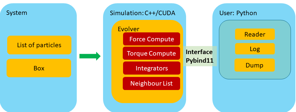
The interface: pybind11
pybind11 is a lightweight header-only library that provide a fast development interface to create Python bindings to existing C++ code. Here we supply a brief description of how to build a Python interface to our C++ ABP code.
pybind11 library has an excellent documentation, so for brevity here we are only focus in how to expose classes and functions. Let us give several concrete examples of how to expose C++ code to Python.
1. Exposing functions
Consider the following C++ function that applies periodic boundary conditions.
///<! @file: enforce_periodic.hpp

inline double enforce_periodic(const double &r, const double &L, const bool& periodic)
{
    double _r = r;
    if (periodic)
    {
        if (_r > 0.5*L)
            _r -= L;
        else if (_r < -0.5*L)
            _r += L;
    }
    return _r;
}
Now, to expose double enforce_periodic(const double &r, const BoxType &box) to Python we need a .cpp file with the following additional lines of pybind11 code:
///<! @file: python_bindings_export.cpp
#include <pybind11/pybind11.h>    ///<!Include the pybind11 library
#include "enforce_periodic.hpp"   ///<!Include enforce_periodic.hpp

PYBIND11_MODULE(cppmodule, m)
{
    m.doc() = "pybind11 example";  ///<! optional module docstring
    m.def("enforce_periodic", &enforce_periodic, "Enforce periodic boundary conditions");
}
The PYBIND11_MODULE() macro creates a function that can be called from within Python. The first argument in PYBIND11_MODULE() is the module name (cppmodule, in our case, whereas the second macro m defines a variable of type py::module which is the main interface for creating bindings. Next, module::def() keyword generates binding code that exposes the enforce_periodic() function to Python. Now from the Python side we can simply write
from cppmodule import *

L = 10.0
x = 11.0
#New x
x_periodic = enforce_periodic(x, L, True)
2. Exposing structured types
Structured types are classes that contain only encapsulated data types such our struct Particle :
///<! @file: particle.hpp

/* @brief 1D particle type */
struct Particle
{
    int id;           // particle id
    int type;         // particle type
    real radius;      // particle radius
    real r;           // particle position
    real v;           // particle velocity
    real f;           // particle force
    real n;           // particle director
};
The following code shows how to expose such a structure to Python. Before we do this, we need to understand how to expose classes with pybind11.
///<! @file: pybind_export_particle.hpp

#include "particle.hpp"

void export_ParticleType(py::module &m)
{
    py::class_<Particle>(m, "Particle")
        .def(py::init<>())
        .def_readwrite("id", &Particle::id, "Particle id")
        .def_readwrite("type",  &Particle::type, "Particle material type")
        .def_readwrite("radius", &Particle::radius, "Particle radius")
        .def_readwrite("r", &Particle::r, "Particle positions")
        .def_readonly("v", &Particle::v, "Particle velocity")
        .def_readonly("f", &Particle::f, "Particle force");
        .def_readwrite("n", &Particle::n, "Particle director");
}
Here the class_ creates bindings for a C++ class or struct-style data structure, and as Python classes. The init() takes the types of a constructor’s parameters as template arguments and wraps the corresponding class constructor. In our case struct Particle doesn't define any constructor inside of C++ code but by using pybind it is possible to extend this without modifying the particle.hpp file
///<! @file: pybind_export_particle.hpp

//..
{
    py::class_<Particle>(m, "Particle")
        .def(py::init<>())  ///<!default constructor
        .def("__init__", [](Particle &self, const int& id, const int& type, const real& radius, const real& r, const real& n) ///<! pybind constructor
             {
                    new (&self) Particle();
                    self. = x;
                    self.y = y;
                    self.id = id;              // particle id
                    self.type = type;          // particle type
                    self.radius = radius;      // particle radius
                    self.r = r;                // particle position
                    self.n = n                 // particle director
                    self.v = 0.0               // particle velocity
                    self.f = 0.0               // particle force
                })
        //..
}
Finally we need to export the Particle type as follows
///<! @file: python_bindings_export.cpp
#include <pybind11/pybind11.h>           ///<!Include the pybind11 library
#include "enforce_periodic.hpp"          ///<!Include enforce_periodic.hpp
#include "pybind_export_particle.hpp"    ///<!Include pybind_export_particle.hpp

PYBIND11_MODULE(cppmodule, m)
{
    m.doc() = "pybind11 cppmodule";                                                       ///<! optional module docstring
    m.def("enforce_periodic", &enforce_periodic, "Enforce periodic boundary conditions"); ///<! export enforce periodic function
    export_ParticleType(m);                                                               ///<! export Particle type
}
Now from the Python side we simply write
from cppmodule import *

p = Particle() # define an empty particle
p.id = 0
p.type = 0
p.radius = 1.0
p.x = 0.35
p.n = -1.0
p.f = -1.2 # Error read only variable!
# and so on ..
# or simple
p = Particle(0, 0, 1.0, 0.35, 1)
3. Export any type of class.
To export a full C++ class containing both member data and member functions, we need to simply follows the steps 1 and 2 taking in account the following
As an example consider the SystemClass defined in ABPTutorial/c++/cppmd/md/system.hpp,
void export_SytemClass(py::module &m)
{
    py::class_<SystemClass>(m, "System")
        .def(py::init<const BoxType &>())
        .def(py::init<const host::vector<ParticleType> &, const BoxType &>())
        .def("get_particles", &SystemClass::get)
        .def("add", &SystemClass::add_particle)
        .def("apply_periodic", &SystemClass::apply_periodic)
        .def("box", &SystemClass::get_box)
        .def_readonly("Numparticles", &SystemClass::Numparticles)
        ;
}
Working Example
Now that we have all key ingredients in place, we can proceed to test our C++ simulation and its Python interface. Before we do this, let us briefly recapitulate the key steps in performing any particle-based simulation.
Review on particle-based simulation
Our simulation workflow consists of three steps:
- Creating the initial configuration;
- Executing the simulation;
- Analyzing the results.
Where, the step 1 feeds into step 2, which, in turn feeds into step 3. The step 1 generate the system configuration for our simulation as a single JSON file (see Python/pymd/builder or ABPTutorial/c++/cppmd/builder).
Let us start with a working example of a full simulation.
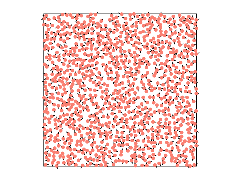
We read the initial configuration stored in the file init.json with $N=4,000$ randomly placed particles in a square box of size $L=100$. We assume that all particles have the same radius $a=1$. Further, each particle is self-propelled with the active force of magnitude $\alpha=1$ and experiences translational friction with friction coefficient $\gamma_t = 1$. Rotational friction is set to $\gamma_r = 1$ and the rotational diffusion constant to $D_r = 0.1$. Particles within the distance $d=2$ of each other experience the polar alignment torque of magnitude $J=1$.
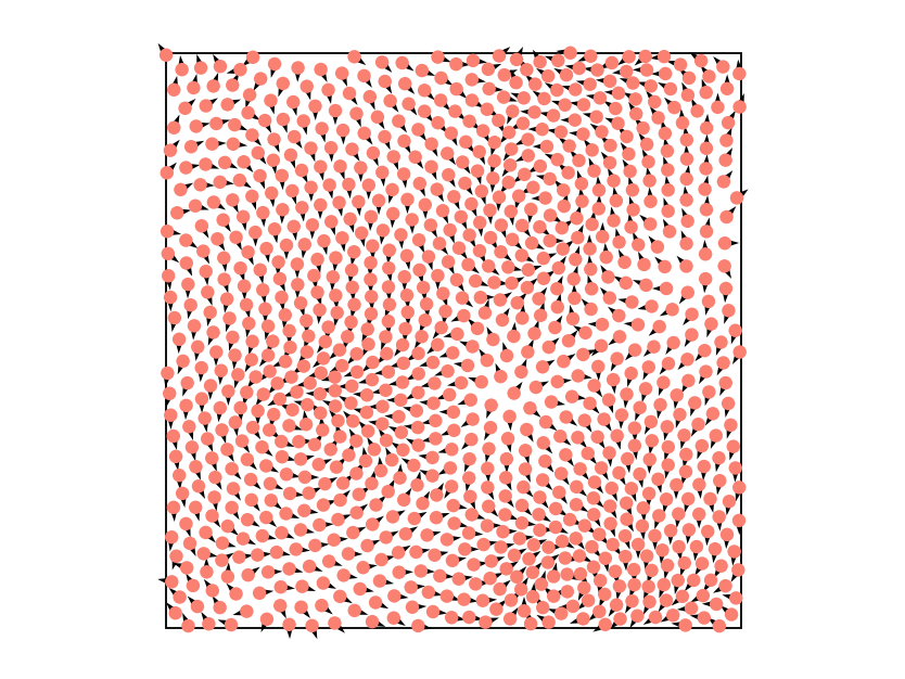
We use the time step $\delta t = 0.01$ and run the simulation for $1,000$ time steps. We record a snapshot of the simulation once every 10 time steps.
%matplotlib widget
import cppmd as md

#particles, box = md.read_json("initphi=0.4L=50.json") #here we read the json file in python
#system = md.System(particles, box)

reader = md.fast_read_json("initphi=0.4L=50.json")  #here we read the json file in c++
system = md.System(reader.particles, reader.box)

dump = md.Dump(system)          # Create a dump object
print("t=0")
dump.show()                     # Plot the particles with matplotlib

evolver = md.Evolver(system)    # Create a system evolver object

#add the forces and torques

# Create pairwise repulsive interactions with the spring contant k = 10 and range a = 2.0
evolver.add_force("Harmonic Force", {"k": 10.0, "a": 2.0})

# Create self-propulsion, self-propulsion strength alpha = 1.0
evolver.add_force("Self Propulsion", {"alpha": 1.0})

# Create pairwise polar alignment with alignment strength J = 1.0 and range a = 2.0
evolver.add_torque("Polar Align", {"k": 1.0, "a": 2.0})

#add integrators
# Integrator for updating particle position, friction gamma = 1.0 , "random seed" seed = 10203 and no thermal noise
evolver.add_integrator("Brownian Positions", {"T": 0.0, "gamma": 1.0, "seed": 10203})

# Integrator for updating particle orientation, friction gamma = 1.0, "rotation" T = 0.1, D_r = 0.0, "random seed" seed = 10203
evolver.add_integrator("Brownian Rotation", {"T": 0.1, "gamma": 1.0, "seed": 10203})

evolver.set_time_step(1e-2) # Set the time step for all the integrators
for t in range(1000):
    #print("Time step : ", t)
    evolver.evolve()    # Evolve the system by one time step
    if t % 10 == 0:     # Produce snapshot of the simulation once every 10 time steps
        dump.dump_vtp('test_{:05d}.vtp'.format(t))
print("t=1000")
dump.show()                     # Plot the particles with matplotlib
Visualizing results
As before, we have saved our output files using the VTP format. For convenience, here we also provide a Paraview state file, which will allow us to rapidly plot the results.
Instructions:
- Open
paraview. - Go to
File->Load State->paraview_plotter.py
If you desire to change the names of the output file or the number/snapshoot steps, you will need to modify the following lines in paraview_plotter.py.
#@file paraview_plotter.py
#...
t0 = 0                       #minimum time step
tf = 1000                    #maximum time step
step = 10                    #snapshot every step
folder = 'your_source_folder'#the source folder
file_name_prefix = 'prefix_' #in our case test_
filenames_vec = [folder+file_name_prefix+'{:05d}.vtp'.format(t) for t in range(t0, tf, step)]
print(filenames_vec)
#...