Session 3
Implementing a 2D simulation of Active Brownian Particles (ABP) in GPUs
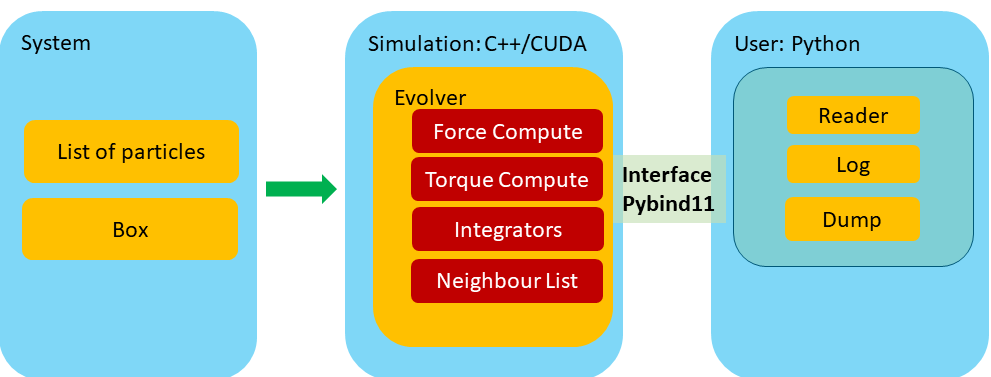
In the second session of this tutorial, we port the C++ and the Python codes developed in Sessions 1 and 2 to modern Graphics Processing Units (GPUs). We keep the structure and naming the same as in the C++ version and only make changes where necessary. We are going to focus on how to implement the force and integrator algorithms in parallel keeping the rest of the code intact.
The figure below outlines the general layout of the simulation package we are developing.
Parallel computing: A brief introduction
Before we dive into the details of the GPU implementation of our simulation, let us briefly overview the basic ideas behind parallel computing, in particular focusing on the use of modern GPUs.
From a practical point of view, parallel computing can be defined as a form of computation in which many calculations are executed simultaneously. Large problems can often be divided into smaller ones, which are then solved concurrently on different computing resources.
Sequential vs Parallel
As we've seen in the previous tutorials, a computer program consist of a series of operations that performs a specified task. For example, our evolve step in the Evolver class needs to perform sequentially the following calculations:
- Check if neighbor list needs rebuilding
- Perform the pre-integration step, i.e., step before forces and torques are computed
- Apply periodic boundary conditions
- Reset all forces and toques
- Compute all forces and torques
- Perform the second step of integration
- Apply period boundary conditions
In general, one can classify the relationship between two pieces of computation as those that are:
(a) related by a precedence restraint and, therefore, must be calculated sequentially, such as the evolve step, and
(b) not related by a precedence restraints and, therefore, can be calculated concurrently. Any program containing tasks that are performed concurrently is a parallel program.
Parallelism
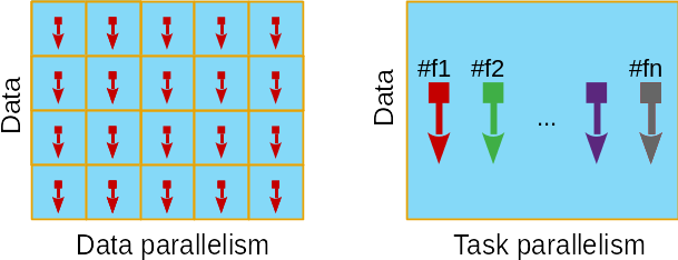
There are two fundamental types of parallelism:
- Data parallelism: when there are many data items that can be operated on at the same time.
- Task parallelism: when there are many tasks that can be operated independently and largely in parallel.
In this final session of this tutorial, we are going to focus on Graphics Processing Units or GPUs, which are especially well-suited to solve problems that can be expressed as data-parallel computations.
GPUs computing: Heterogeneous Architecture
Nowadays, a high-end workstation or a typical compute node in a high-performance computer cluster contains several multi-core central processing unit (CPU) sockets and one or more GPUs. The GPU acts a co-processor to a CPU operating through a PCI-Express BUS. GPUs are designed to fulfill specialized task, in particular, for producing high-resolution graphics in real time. A modern GPU consists of several thousands compute cores.
In terms of its purpose, a CPU core is designed to optimize the execution of sequential programs. In contrast, a GPU core (much simpler in design than a CPU core) is optimized for data-parallel tasks focusing on the large throughput. Since the GPUs function as a "co-processor", the CPU is called the host and the GPU is called the device.
Because of this host-device relationship, any GPU-based application consist of two parts:
- Host code
- Device code
As the name suggests, the host code is executed on the CPU, while the device code runs on GPUs. Typically, the CPU is in charge of initialize the environment for the GPU, i.e, allocating memory, copying the data, etc.
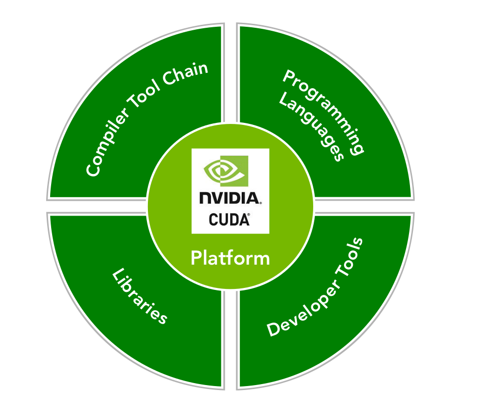
The CUDA platform
CUDA is a parallel computing platform and programming model that makes use of the parallel compute engine of NVIDIA GPUs. From the practical point of view, CUDA provides a programming language interface for C, C++, Fortran, openCL programming languages.
The CUDA Programming Model
Here we are going to briefly overview how to write CUDA-C/C++ code that makes use of the GPU. As stated above, our application consist in two "types" of code. The first is the host code and the second is the device code. The device code (which is exclusively executed on the GPU) is denominated kernel. The kernels function are identified by the keyword __global__, and by the fact that never return any value (i.e., they always have the void return type). The following example shows a simple Hello, world! program:
//@file: hello_world.cu
#include "hello_world.hpp"

// device code start
__global__ void hello_world_kernel()
{
    printf("hello");
}
// device code end

// host code start
void call_hello_world_kernel(void)
{
    hello_world_kernel<<<1,1>>>();
    cudaDeviceSynchronize (); //Wait for compute device to finish.
                              //forcing printf to flush
}
// host code end

//@file: hello_world.hpp
void call_hello_world_kernel(void); //forward declaration

//@file: main.cpp
#include "hello_world.hpp"

// host code start
int main()
{
    ///...

    call_hello_world_kernel();

    ///...
}
// host code end
Kernels codes have several properties:
- are identified by the
__global__qualifier withvoidreturn type; - are only executable on the device;
- are only callable by the host.
Where is the parallelism here?
So far we haven't seen any parallelism. Before we can do this, we need to understand two fundamental concepts in the CUDA-verse:
- Thread abstraction and organization;
- Memory hierarchy.
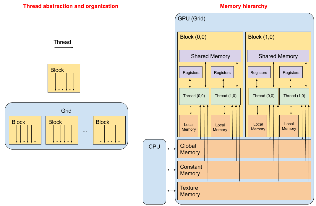
1. Thread abstraction and organization
Kernels need to be configured to be run on the device. In the previous code, the triple chevrons<<<X, Y>>> represents the execution configuration, that dictates how many device threads execute the kernel in parallel. A thread of execution is the smallest sequence of programmed instructions that can be managed independently. In CUDA, all threads essentially execute the same piece of code: thread abstraction.
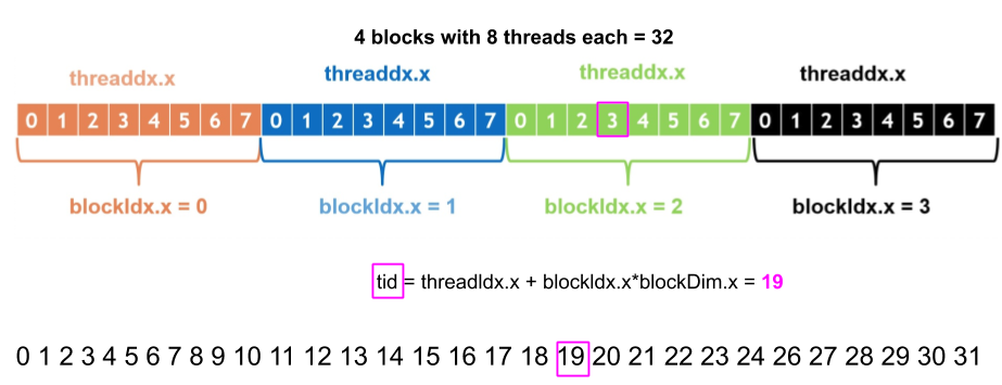
A single invoked kernel is referred to as a grid. A grid is comprised of thread blocks. A block is comprised of multiple threads. In the CUDA programming model, we speak of launching a kernel with a grid of thread of blocks. The first argument in the execution configuration (<<<X, Y>>>) specifies the number of thread blocks in the grid, and the second specifies the number of threads in a thread block.
//@file: hello_world.cu
#include "hello_world.hpp"

// device code start
__global__ void hello_world_kernel()
{
    int tid = blockIdx.x*blockDim.x + threadIdx.x;
    printf("hello <global> thread id=%i block id=%i <local> thread id=%i", tid, blockIdx.x, threadIdx.x);
}
// device code end

// host code start
void call_hello_world_kernel(void)
{
    uint thread_of_blocks = 4;
    uint threads_in_block = 8;

    hello_world_kernel<<<thread_of_blocks,threads_in_block>>>();
    cudaDeviceSynchronize (); //    Wait for compute device to finish.
    //here hello will be printed $thread_of_blocks \times threads_in_block = 32$
}
// host code end
Example:
2. Memory hierarchy
CUDA programming model expose on-chip memory hierarchy allowing the user to make an efficient use of the resources to speed up applications. In general the memory can be programmable and non-programmable. L1 cache and L2 cache in the CPU memory space, are examples of non-programmable memory. On the other hand, the CUDA memory model exposes many types of programmable memory: Registers, Shared memory, Local memory, Constant memory, Texture memory, and Global memory (see figure above). In this tutorial, we are going to cover some aspects of the Global memory and the Constant memory.
Global memory Is the largest, highest-latency, and most commonly used memory on a GPU. Its state can be accessed from the device throughout the lifetime of the application. A variable in global memory can either be allocated statically or dynamically.
Constant memory As the name may indicate, we use constant memory for data that will not change over the course of a kernel execution.
Example: $v_{i}=i\,a+b$
//@file: hello_world.hpp

// Global memory statically in device code using the qualifier __device__
__device__ int my_static_variable = 2;

__device__ int my_static_variable_vec[10];


// Constant memory statically in device code using the qualifier __constant__
__constant__ int my_const_static_variable = -1;


void call_hello_world_sum_kernel(void); //forward declaration

//@file: hello_world.cu
#include "hello_world.hpp"

// device code start
__global__ void hello_world_sum_kernel(__constant__ int Num, int* vector_of_int_dev)
{
    int tid = blockIdx.x*blockDim.x + threadIdx.x;
    //For cases where the number of elements in the arrays is not evenly divisible by the thread block size
    //the kernel code must check for out-of-bounds memory accesses
    if(tid<Num)
    {
        vector_of_int_dev[tid] = tid*my_static_variable + my_const_static_variable;
    }
    //..
}

// host code start
void call_hello_world_sum_kernel(const unsigned int Num = 100)
{
    ///dynamically
    unsigned int nbytes = Num * sizeof(int);

    // allocate the host memory
    int *vector_of_int_host = (int *)malloc(nbytes);

    // allocate the device vector
    int *vector_of_int_dev;
    cudaMalloc((int **)&vector_of_int, nbytes);

    // initialize the host vector
    for(unsigned int i=0;i<Num;i++) vector_of_int_host[i] = 0;

    // transfer data from the host to the device
    cudaMemcpy(vector_of_int_host, vector_of_int_dev, nbytes, cudaMemcpyHostToDevice);

    //Do something with the vector_of_int_dev
    do_something<<<(Num+255)/256, 256>>>(vector_of_int_dev);


    // transfer data from the device to the host
    cudaMemcpy(vector_of_int_host, vector_of_int_dev, nbytes, cudaMemcpyDeviceToHost);

    // free memory
    cudaFree(vector_of_int_dev);
    free(vector_of_int_host);

}
// host code end
CUDA Libraries: Thrust
As in C/C++, native CUDA libraries provide collection of function definitions whose signatures are exposed through header files. The CUDA libraries are special in that all computation implemented in the library is accelerated using a GPU.
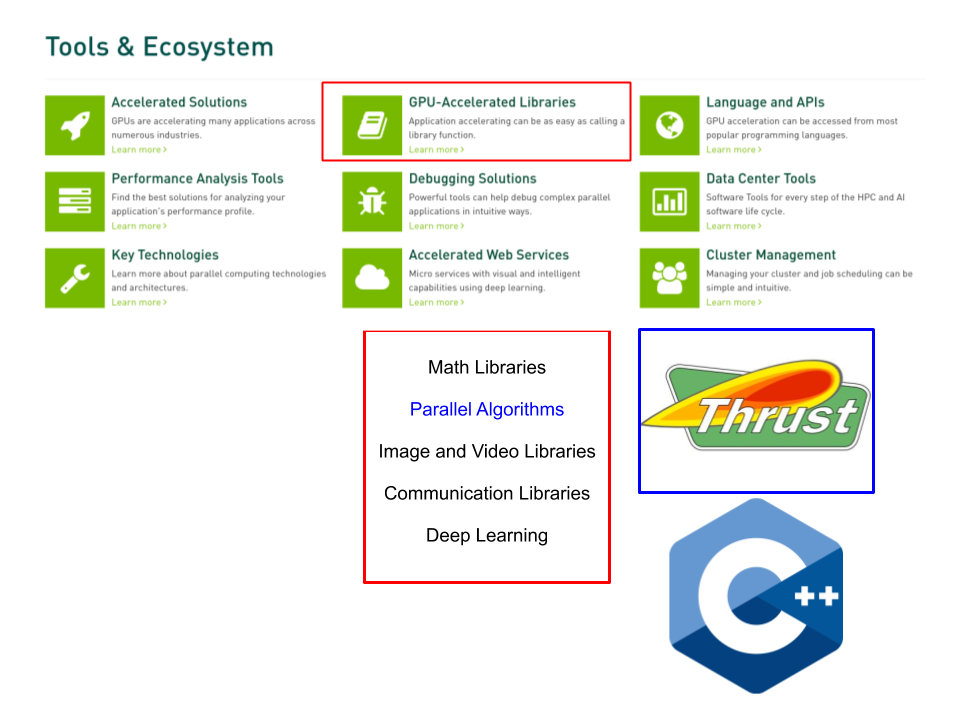
In the provided code, we have made a full use of thrust as a replacement for Standard Template Library (STL) library. Thrust is a C++ template library for CUDA based on the STL that allows to implement high performance parallel applications with minimal programming effort through a high-level interface. For example, in our previous example we manually allocate memory on the device by calling cudaMalloc (void **devPtr, size_t size) then we copy the host data to the device by using cudaMemcpy( void * dst, const void *src, size_t count, enum cudaMemcpyKind kind ), and finally at the end of the execution we free the memory by calling cudaFree(devPtr). Using Thrust we need to simply do:
#include <vector> //stl vector
#include <thrust/device_vector.h> //thrust vector
#include <thrust/copy.h>          //thrust copy

{
    //...
    //allocate & initialize the host vector
    std::vector<int> vector_of_int_host{Num, 0};

    //allocate & copy the device vector
    thrust::device_vector<int> vector_of_int_dev = vector_of_int_host;

    //or we can simple do
    thrust::device_vector<int> vector_of_int_dev{Num, 0};

    //Do something with the vector_of_int_dev
    do_something<<<(Num+255)/256, 256>>>(device::raw_pointer_cast(&vector_of_int_dev[0]));

    //device::raw_pointer_cast creates a "raw" pointer from a pointer-like type, simply returning the wrapped pointer
    // pretty much like *vector_of_int_dev

    // stl like copy to vector_of_int_host
    thrust::copy(vector_of_int_dev.begin(), vector_of_int_dev.end(), vector_of_int_host.begin());

    //DONE! We don't need to free memory since is managed by thrust
}
For more information please check ~/cuda/gpumd/md/src/types/devicevector.hpp**
Real world example: The harmonic force calculation
Let's compare the harmonic force implementation in CPU harmoniccpp.cpp versus the GPU one harmoniccuda.cpp:
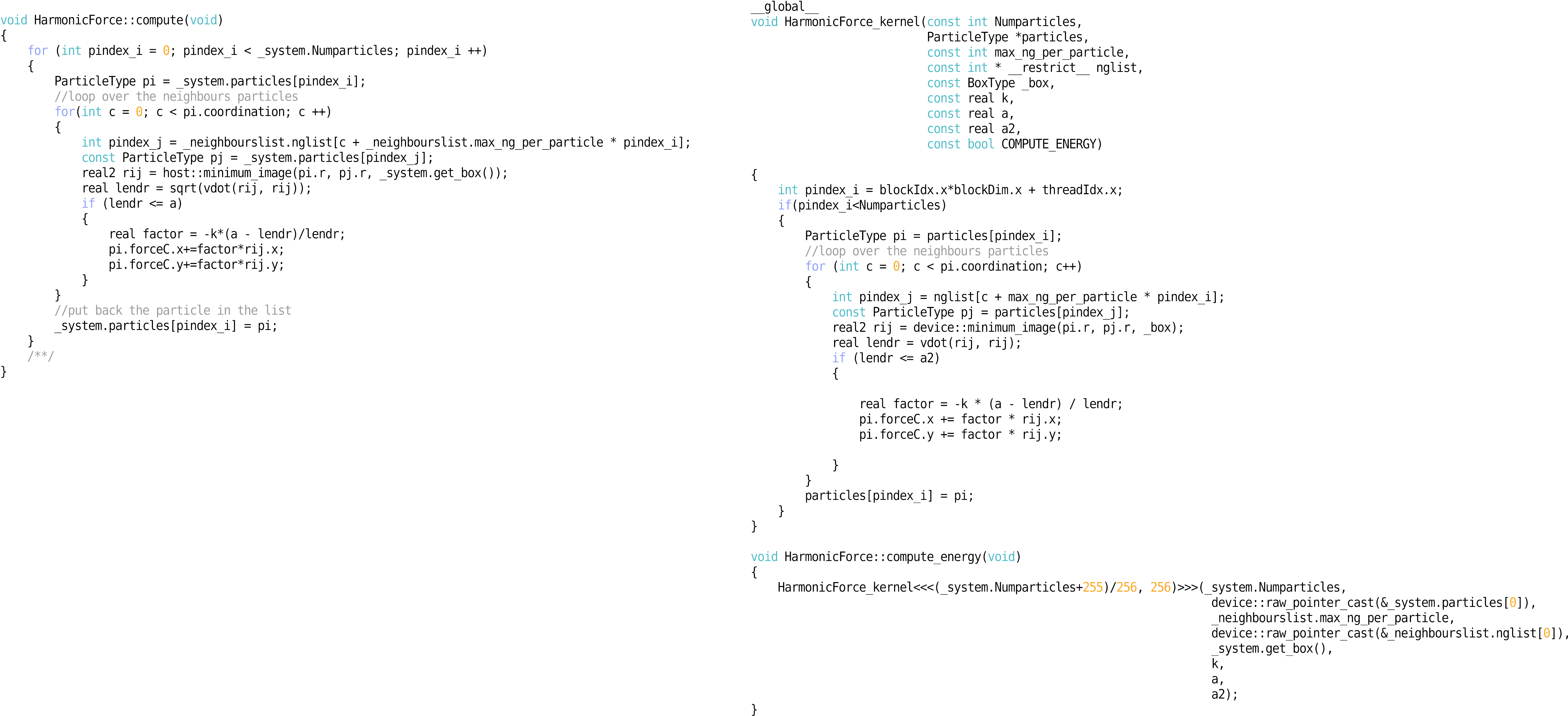
By now, we should all be familiar with the cppmd package developed in the Session 2. Let's take a closer look into what have changed when switching to GPUs:
- the
std::vector<T>were replaced bythrust::device_vector<T>. - there is a kernel function
void HarmonicForce_kernel(...)that calculate the forces for each particle in parallel by replacing the for loop on the right (3). - for loop is now replaced by:
{
 int pindex_i = blockIdx.x*blockDim.x + threadIdx.x;
 if(pindex_i<Numparticles)
 {
     ///...
 }
}
That's all! The rest of the code remains unchanged!
Conclusion
Note that the code presented here could be further optimized for running on GPUs. For example, the HarmonicForce_kernel have several irregular memory access pattern where different threads read the same memory bank, e.g., each particle has more than one neighbor and each of those neighbors needs the information stored in particle j to calculate the force. This results in serialization during reading, which affect the performance. To fix this, one should make use Memory hierarchy (shared memory would do the trick in this case!) which is out of scope on this tutorial.
One of the drawbacks of parallel computation is that hardware and software deployment are deeply intertwined. This means that in order to optimize the code we first need to have a deep understanding of how hardware operates, like in Memory hierarchy case. Nevertheless, even with the basic parallel application implementation we can gain significant speed-ups.
Code optimization
Follow common sense! Let's say that a given application is 5x faster compared to the serial code and after "deep" optimization that would take weeks to implement and make the code "harder" to maintain you only gained 7x speedup with respect to the serial code, then the effort is not worth it.
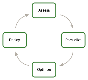
Assess, Parallelize, Optimize, Deploy (APOD)
APOD is a cyclical process: initial speedups can be achieved, tested, and deployed with only minimal initial investment of time, at which point the cycle can begin again by identifying further optimization opportunities, seeing additional speedups, and then deploying the even faster versions of the application into production.
Working Example
Now that we have all key ingredients in place, we can proceed to test our CUDA implementation and its Python interface. Before we do this, let us briefly recapitulate the key steps in performing any particle-based simulation.
Review on particle-based simulation
Our simulation workflow consists of three steps:
- Creating the initial configuration;
- Executing the simulation;
- Analyzing the results.
Let us start with a working example of a full simulation.
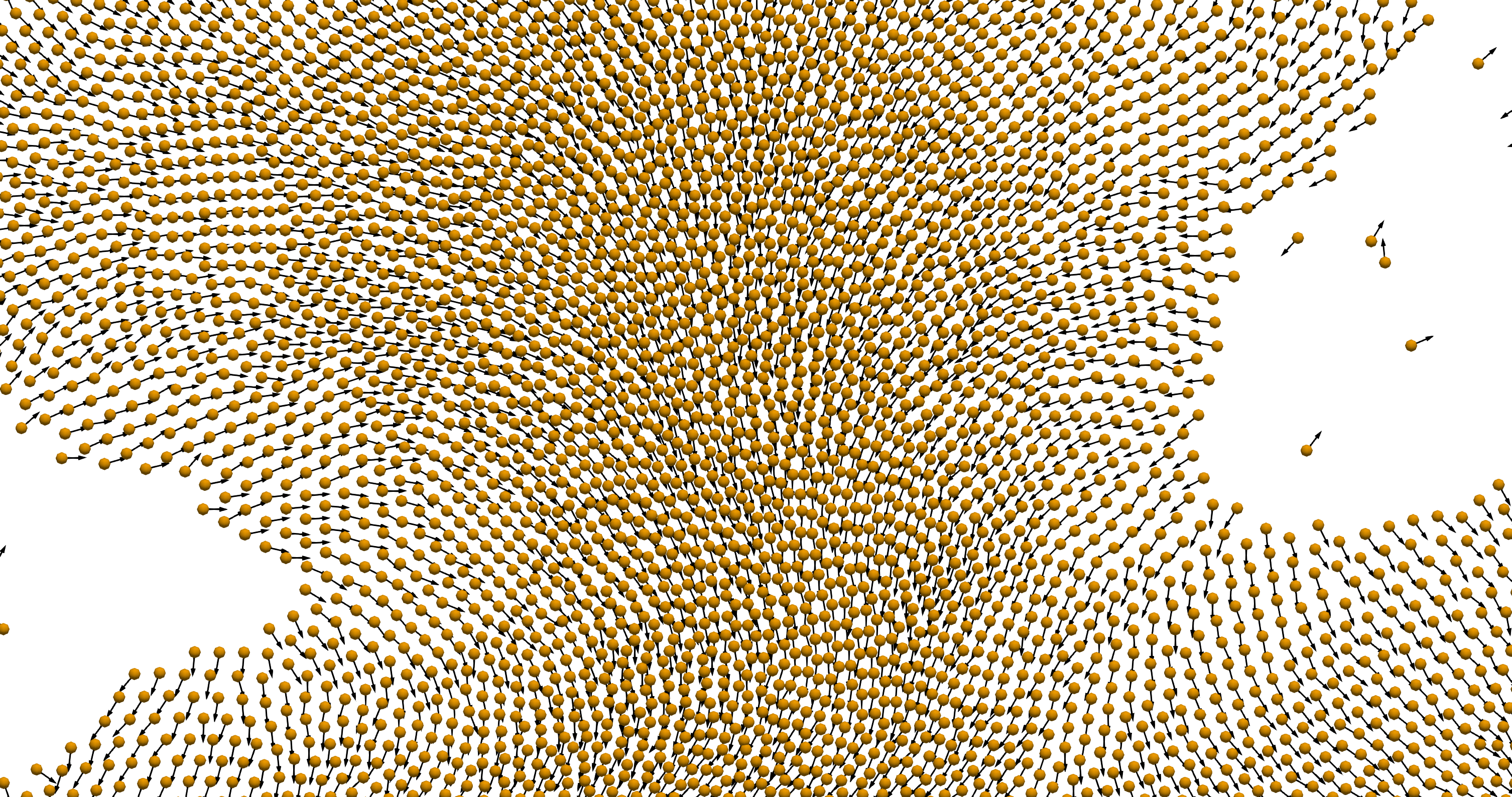
We read the initial configuration stored in the file init.json with $N=36,000$ randomly placed particles in a square box of size $L=300$. We assume that all particles have the same radius $a=1$. Further, each particle is self-propelled with the active force of magnitude $\alpha=1$ and experiences translational friction with friction coefficient $\gamma_t = 1$. Rotational friction is set to $\gamma_r = 1$ and the rotational diffusion constant to $D_r = 0.1$. Particles within the distance $d=2$ of each other experience the polar alignment torque of magnitude $J=1$.
We use the time step $\delta t = 0.01$ and run the simulation for $1,000$ time steps. We record a snapshot of the simulation once every 10 time steps.
%matplotlib widget
import gpumd as md
import time

json_reader = md.fast_read_json("initphi=0.4L=300.json") #here we read the json file in C++
system = md.System(json_reader.particles, json_reader.box)

#get the GPU hardware properties
cuda_info = system.get_execution_policies()
print("** Device parameters **")
print(cuda_info.getDeviceProperty())
print("** Lunch parameters **")
print("GridSize=", cuda_info.getGridSize(), "BlockSize=", cuda_info.getBlockSize())
dump = md.Dump(system)          # Create a dump object
print("t=0")
#dump.show(notebook=True)        # Plot the particles with matplotlib

evolver = md.Evolver(system)    # Create a system evolver object

#add the forces and torques

# Create pairwise repulsive interactions with the spring contant k = 10 and range a = 2.0
evolver.add_force("Harmonic Force", {"k": 10.0, "a": 2.0})

# Create self-propulsion, self-propulsion strength alpha = 1.0
evolver.add_force("Self Propulsion", {"alpha": 1.0})

# Create pairwise polar alignment with alignment strength J = 1.0 and range a = 2.0
evolver.add_torque("Polar Align", {"k": 1.0, "a": 2.0})

#add integrators
# Integrator for updating particle position, friction gamma = 1.0 , "random seed" seed = 10203 and no thermal noise
evolver.add_integrator("Brownian Positions", {"T": 0.0, "gamma": 1.0, "seed": 10203})

# Integrator for updating particle orientation, friction gamma = 1.0, "rotation" T = 0.1, D_r = 0.0, "random seed" seed = 10203
evolver.add_integrator("Brownian Rotation", {"T": 0.1, "gamma": 1.0, "seed": 10203})

evolver.set_time_step(1e-2) # Set the time step for all the integrators

start_clock = time.time()
for t in range(10000):
    #print("Time step : ", t)
    evolver.evolve()    # Evolve the system by one time step
    #if t % 10 == 0:     # Produce snapshot of the simulation once every 10 time steps
    #    dump.dump_vtp('test_{:05d}.vtp'.format(t))
print('36000 particles - 10000 steps execution time {:.2f}[s]'.format(time.time() - start_clock))
print("t=10000")
#dump.show(notebook=True)              # Plot the particles with matplotlib

Speed up comparison
Now let's see how the GPU code compare with the previous session.
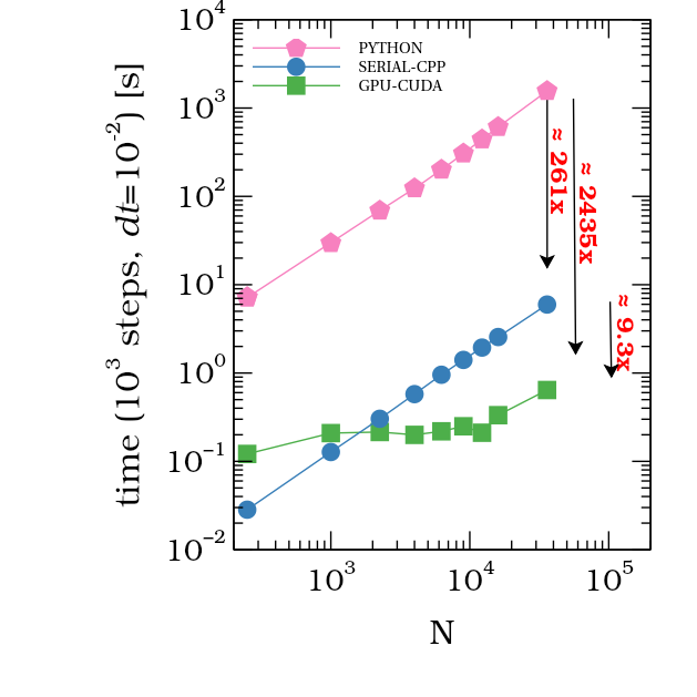
As you can see, even the first round on the Assess, Parallelize, Optimize, Deploy give us 2435x times faster than the Python code, and 9.3x times than the c++ code.
References
- https://devblogs.nvidia.com/
- https://docs.nvidia.com/cuda/cuda-c-programming-guide
- https://docs.nvidia.com/cuda/cuda-c-best-practices-guide
- Cheng, John, Max Grossman, and Ty McKercher. Professional CUDA c programming. John Wiley & Sons, 2014.
- Jaegeun Han and Bharatkumar Sharma Learn CUDA Programming. Packt Publishing, 2019.